DileepReddy

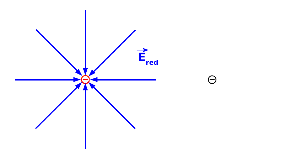
All first courses on electromagnetism introduce Coulomb’s expression for the electric field due to a point charge. Given an electron with charge \(-q\), the field at a distance \(r\) away would read \[\mathbf{E} = \frac{-q}{4\pi\epsilon_0r^2}\hat{\mathbf{e}}_{\mathbf{r}}.\]

Thus, if another electron were to be placed at said location at a distance \(r\) from the first one, it would experience the existence of the first electron as a repulsive force, albeit diminished in magnitude due to distance.

What if one were to move the first electron? How soon would the second electron detect this change? And in what manner?

It is possible (though not necessarily useful) to reduce all of Maxwell’s equations into a form well suited for discussing point charges such as these. To quote from Richard P. Feynman’s “Lectures on Physics Vol. I,” chapter 28, the full form looks like \[\mathbf{E}= \frac{-q}{4\pi\epsilon_0}\left[\frac{\hat{\mathbf e}_{\mathbf r'}}{r'^2} + \frac{r'}{c}\frac{d}{dt}\left(\frac{\hat{\mathbf e}_{\mathbf r'}}{r'^2}\right)+\frac{1}{c^2}\frac{d^2}{dt^2}\hat{\mathbf e}_{\mathbf r'}\right].\]

The little prime on \(r\) is meant to account for the time-delay for information to travel from the electron to the measurement point. \(r'\) is the retarded distance, and \(\hat{\mathbf e}_{\mathbf r'}\) the apparent direction pointing towards where the source electron was located at a time \(r'/c\) ago.

The first two terms are merely the Coulombic field, and a first-order temporal correction to it. The both of them scale as \(1/r^2\), and can be neglected at large distances. The third term, however, depends on the transverse/lateral acceleration (i.e. perpendicular to the line-of-sight) of the source electron, and falls off with distance, at a rate slower than the Coulombic terms: \[E_\perp = \frac{-q}{4\pi\epsilon_0c^2r}a_\perp\left(t-\frac{r}{c}\right).\]

This indicates that the electromagnetic field has a sluggish quality to it that causes rapid disturbances to spread out in space at speed \(c\). It also implies that accelerating charges radiate energy. We see this in synchrotron radiation, and use it in free-space communication technologies. The slow, \(1/r\) fall-off is also the reason light emitted by electronic motion in a galaxy 5 billion light-years away can be picked up by CCD detectors here on earth.

In practice, it is rather difficult to isolate a single electron, and then cause it to accelerate, and subsequently detect its radiation. However, note that the radiative component of the electric field is separate from the Coulombic components, which can be cancelled by an inertial positive charge placed at the right location. Meaning, we can generate radiation by inducing a bulk acceleration of several free (conductive) electrons in a neutral wire of metal, as is done in typical transmission antennae.

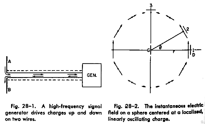
Applying a simple, monochrome Sine-wave voltage across a straight metal rod would generate an oscillating dipole field in its vicinity. The efficiency with which said dipole antenna would radiate energy away depends on the length of the rod relative to the wavelength of light at that Sine-wave frequency (a la impedence-matching), but the basics of our field formula would still hold. If the dipole were aligned along the z-axis in polar coordinates, then the field amplitude would fall off as \(1/r\), irrespective of the azimuthal angle \(\phi\). But because the field depends on the transverse acceleration of the charges perpendicular to the line of sight, the polar (\(\theta\)) dependence would be a simple Cosine-projection, and would vanish directly above or below the rod.

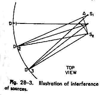
The field structure becomes more interesting when we place two dipole antennae in parallel (at locations \(S_1\) and \(S_2\) in the above figure), and drive them in sync with the same Sine-wave voltage. Naturally, the both of them would produce their own independent, oscillating-dipole electric fields. The total field would be the vector-sum of the two. And because the fields are sinusoidal, receivers at different locations (\(D_1\), \(D_2\), \(D_3\)) would experience the two fields retarded by different amounts, based on the relative distances. Consequently, the two waves would add constructively in some directions, and destructively in others.

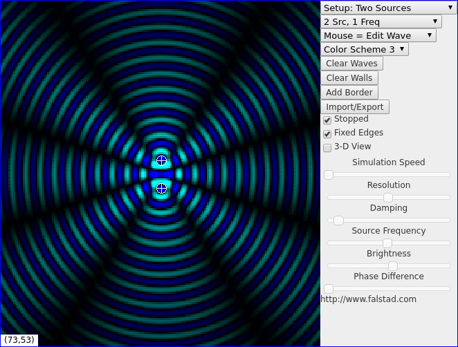
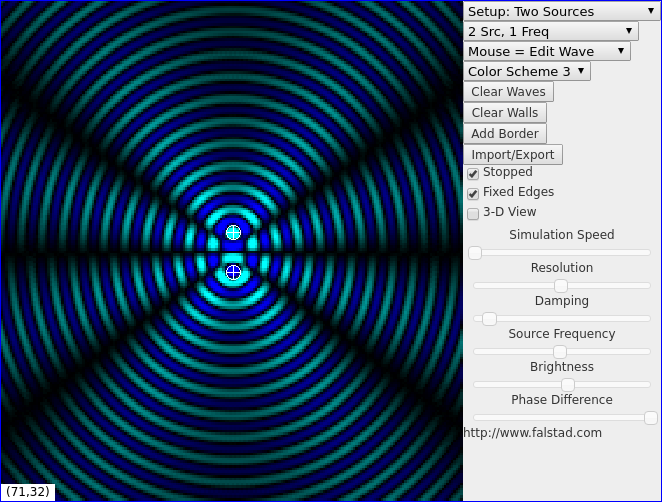
The number of hotspot (and cancellation deadzone) sectors around the two antennae is determined by the distance between them, relative to the wavelength of the frequency in question. In the above image, for example, the dipoles are being driven in-phase (i.e. together), and are placed two wavelengths apart. The resulting field distribution is essentially the Young’s double-slit interference pattern. We can swap the hotspots with the deadzones by merely shifting one of the dioples in phase by \(180^\circ\) relative to the other, as shown below.

To illustrate the addition of monochrome Sine-waves better, I have created these one-dimensional, unidirectional, toy animations of dipole radiators and receivers. For further simplicity, the \(1/r\) decay of the amplitude has also been neglected. If two sources (red and blue) were placed two wavelengths apart and driven in-phase (in sync), then the receiver (green) would indeed see a coherent sum of the two individual waves.

If the sources were to be driven out of phase, then naturally, in the collinear direction, the waves would cancel each other.

Another way to destructively interfere in the collinear direction while still being driven in-phase is to separate the sources by a distance that is an integer number of wavelengths plus half-a-wavelength, as below.

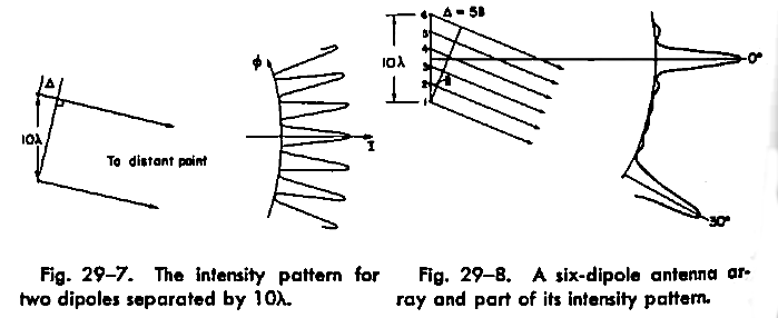
Of course, the next obvious step is to add more antennae. Still sticking to the simple, one-dimensional picture, one can cause a regularly spaced array of dipole antennae to constructively interfere in the collinear direction, if their relative phases are connect for their relative positions. For instance, antennae separated by a whole number of wavelengths have to oscillate in phase, and those separated by a whole number plus half-a-wavelength have to oscillate out of phase, as shown below. The principle carries over to arbitrary separations as well.

If we return to the two-dimensional, in-plane radiation pattern, we will observe a more complex fringe structure than mere two-slit interference. For example, if we had six radiators (like below), then there would be fewer directions in which all six dipole patterns would add constructively. Consequently, all the output power would be concentrated into narrow sectors along special directions determined by the exact seperation and relative phases. The more antennae we add, the more knobs we have to play with (positions of said antennae, power, phase, and orientation of each, etc.), the better our control over the radiation pattern. This is the basic concept behind phased arrays.

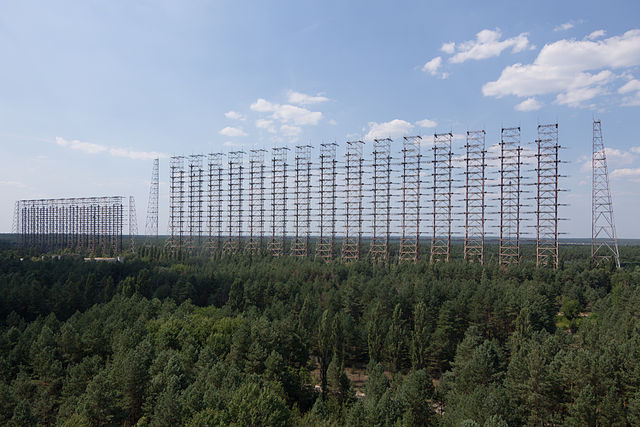
The radiation pattern of an antennae array is identical to it’s sensitivity plot. In other words, if a giant array of antennae were all to receive a single-frequency (monotone) signal, then the relative phases of the signals from each subcomponent of the array can reveal the exact direction of it’s origin (up to the resolution of the array, which depends on the size of the array, etc.). This is how large arrays of radio telescopes pinpoint the sources of cosmic signals without having to move much. Perhaps the best use case of antennae arrays is in radars, where they are used to both transmit and receive. And the most famous example for one of these is the fabled Russian Woodpecker.

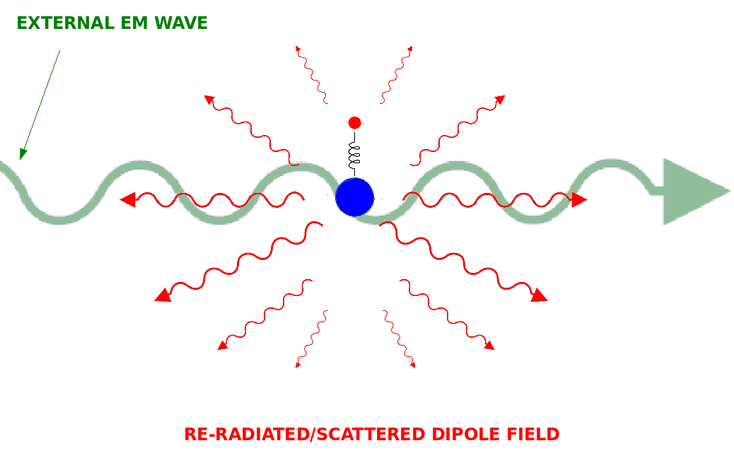
So much for large antennae. We now move on to tiny atoms. Ever since Fraunhofer (and Wollaston before him) discovered dark depressions in the solar spectrum in the early 19th century, we’ve known about special absorption frequencies for various materials. Over two centuries worth of work has lead to a pretty solid theory to explain these as electronic transitions between energy levels. However, we are concerned with how atoms behave when excited at frequencies far away from any of its absorption lines. That is, what happens when an electromagnetic wave of frequency that is not resonant with any electronic transition within an atom, excites it? A good model for the atom’s behavior turns out to be a simple, classical particles on a spring!

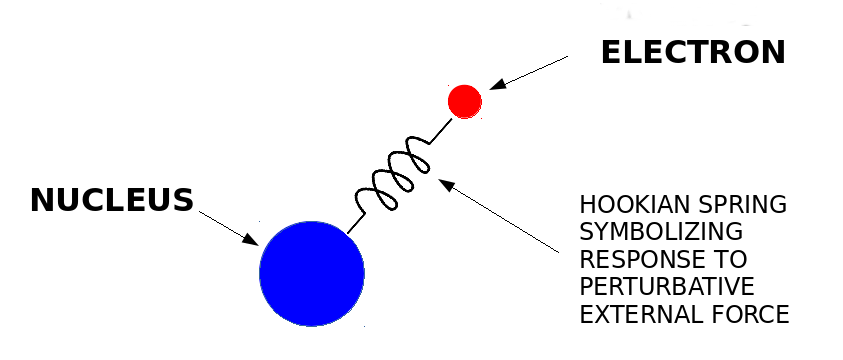
The heavy nucleus is unlikely to respond much to a weak, external wave. The electrons, however, get easily knocked around. If the external, non-resonant field isn’t too strong, the electrons in a free, gaseous atom will simple oscillate about the nucleus at a matching frequency, and along the direction of the polarization of the external field. The atom know behaves like a miniature dipole antenna. The oscillating electron will know lose its energy (due to acceleration) back into the electromagnetic field by radiating in a dipole pattern. This occurs in systems where the atoms/molecules are smaller than the wavelength of the external field, and is called Rayleigh scattering. This is why one can see the path of a laser beam in the fog. And to a large extent, this is also why the sky is blue.

The direction of the re-radiated power from individual atoms has no correlation to that of the external beam (apart from the polarization orientation of the dipole). If we were to consider a whole host of atoms, then the picture changes. For instance, we return to the one-dimensional picture, and place a linear array of atoms as a stand-in for the bulk of a transparent medium. Since we don’t need to restrict ourselves to crystalline media, we can space them randomly as well. But as long as the dipoles are all being driven by the same coherent, external beam, then they will automatically be phased to re-radiate constructively in the “forward” direction of the external beam. With more atoms in the path (i.e. thicker the slab), the less the power scattered in other directions. Therefore, a beam can pass through a slab of glass, or a glass of water, largely unmolested. The energy of the beam has to temporarily be shared between the electromagnetic field, and the eletrons in the medium, however. This leads to some interesting effects that are the subject of the following sections.

(Coming Soon)

(Coming Soon)

(Coming Soon)

(Coming Soon)